Projects for Second-Order Differential Equations

Section 4.5 Projects for Second-Order Differential Equations

Subsection 4.5.1 Project—Tuning a Circuit

Differential equations prove exceptional at modeling electrical circuits.²⁴ In Subsection 4.1.1, we modeled a simple RLC circuit, which is fundamental to larger circuit building. We found that circuits with the three of the most fundamental electrical objects, resistors, capacitors, and inductors, can be modeled by constant coefficient, linear, second order differential equations. Consider the circuit in Figure 4.1.1. We found that the circuit can be modeled by

$\begin{equation} L I'' + RI' + \frac{1}{C} I = E'(t),\label{secondorder05-equation-rlc}\tag{4.5.1} \end{equation}$

🔗

where

$I(t)$ is the current flowing through the circuit,

$E(t)$ is the impressed voltage,

$R$ is the resistance

$R\text{,}$ and

$C$ is the capacitance. Of course we will also need to know

$I(0)$ and

$I'(0)$ if we wich to formulate an initial value problem. Notice that (4.5.1) is very similar to the spring-mass model developed in Subsection 2.1.2,

$\begin{equation*} mx'' + bx' + kx = f(t), \end{equation*}$

🔗

where

$m$ is the mass,

$b$ is the damping coefficient, and

$k$ is the spring constant (Table 4.5.1).

This project is from Brian Winkel (2016), “4-060-S-CircuitTuner,” https://www.simiode.org/resources/2848.

🔗

Table 4.5.1. Comparison of terms between spring-mass and RLC circuit differential equations

Spring-Mass Model	RLC Circuit
mass $m$	inductance $L$
damping $b$	resistance $R$
spring constant $k$	inverse of capacitance $1/C$
forcing function $f(t)$	derivative of induced voltage $E'(t)$

🔗

Subsubsection Simple RLC Circuit Model, Solution, and Interpretation

🔗

We now examine a circuit in which a current is present and does not have a driving

$E(t)\text{,}$ expecting things to dampen out, in this case current to run out. Let us consider an RLC circuit as depicted in Figure 4.1.1 in which we have an initial current,

$I(0) = 3.2$ amps with a resistance of

$R = 7$ ohms, an inductance of

$L = 1$ henry, and a capacitance of

$C = 0.1$ farads. Since we have some current in the circuit already

$I(0) = 3.2$ at the start we shall not need an inducing

$E(t)\text{,}$ so

$E(t) = 0\text{.}$ Let us see what happens to the current in the circuit by solving the appropriate RLC circuit differential equation

$\begin{equation*} 1 \cdot I'' + 7I' + \frac{1}{0.1} I = 0, \quad I(0) = 3.2, \quad I'(0) = 0. \end{equation*}$

🔗

Of course, this initial value problem might be easier analyze in the form,

$\begin{equation} I'' + 7I' + 10 I = 0, \quad I(0) = 3.2, \quad I'(0) = 0.\label{secondorder05-equation-example-rlc}\tag{4.5.2} \end{equation}$

🔗

Activity 4.5.1.

🔗

(a)

Solve the RLC circuit differential equation (4.5.2) for $I(t)\text{.}$ If you use Sage to solve this equation, remember that I is the reserved symbol for $i\text{,}$ the square root of $-1\text{.}$

🔗

(b)

Consider the values of $R$ to be $0.007\text{,}$ $0.07\text{,}$ $0.7\text{,}$ $7\text{,}$ $70\text{,}$ and then $700\text{,}$ and solve (4.5.2) in each case, keeping all other values the same. Plot the solutions for the current in the circuit over the time interval $[0, 25]$ s with a vertical plot interval $[−3, 3]$ in each case. Identify each plot with its associated $R$ value and describe what is happening to the current, $I(t)\text{,}$ in each corresponding circuit over time, $t\text{.}$

🔗

Let us consider the differential (4.5.3) for an RLC circuit with driving voltage

$E(t) = \sin( \omega t)$ (current

$I(t) = y(t)$ ),

$\begin{equation} L y'' + Ry' + \frac{1}{C} y = \omega \cos(\omega t).\label{secondorder05-equation-forced-rlc}\tag{4.5.3} \end{equation}$

🔗

We can use Sage to solve this equation.

xxxxxxxxxx
 
t =var('t');
y = function('y')(t); 
L = var('L'); assume(L < 0)
R = var('R'); assume(R > 5)
C = var('C'); assume(C > 5)
assume(C*R^2 + 4*R^2 - 4*L - 400 >0) 
omega = var('omega'); assume(omega > 0)
DE = L*diff(y,t,2) + R*diff(y,t) + y/C == omega*cos(omega*t)
sol = desolve(DE, y, ivar = t, ics=[0, 0, 0])
sol.show()

🔗

The solution is pretty long, but notice that is the transient solution that approaches zero as

$t \to \infty$ and then there is the steady state solution,

$\begin{equation} y_{\text{steady state}} = \frac{C^{2} R \omega^{2} \sin\left(\omega t\right) - {\left(C^{2} L \omega^{3} - C \omega\right)} \cos\left(\omega t\right)}{C^{2} L^{2} \omega^{4} + {\left(C^{2} R^{2} - 2 \, C L\right)} \omega^{2} + 1}.\label{secondorder05-equation-steady-state}\tag{4.5.4} \end{equation}$

🔗

We would like to study gain, the ratio of the amplitude of the steady state output voltage,

$V_{\text{out}}$ to the amplitude of the input voltage,

$V_{\text{in}}\text{,}$ or

$V_{\text{out}} / V_{\text{in}}\text{.}$ We measure

$V_{\text{out}}$ as the amplitude of the steady state voltage across the resistance

$R$ in the circuit or

$\begin{equation*} V_{\text{out}} = R \cdot \text{Amplitude}(y_{\text{steady state}}(t)). \end{equation*}$

🔗

In our case

$V_{\text{in}}$ is just 1 for

$E(t) = \sin( \omega t)\text{.}$

🔗

Subsubsection Trigonometry Pause and Phase Angle

🔗

The initial value problem

$\begin{equation*} ay'' + by' + cy = 0, \quad y(0) = y_0, \quad y'(0) = 0 \end{equation*}$

🔗

has the following solution when the discriminant

$b^2 - 4ac \lt 0\text{,}$

$\begin{align} y(t) \amp = A e^{-bt/2a} \sin\left( \frac{\sqrt{4ac - b^2}}{2a} t \right) + Be^{-bt/2a} \cos\left( \frac{\sqrt{4ac - b^2}}{2a} t \right)\label{secondorder05-equation-trig-phase-angle}\tag{4.5.5}\\ \amp = e^{-bt/2a} \left( A \sin\left( \frac{\sqrt{4ac - b^2}}{2a} t \right) + B \cos\left( \frac{\sqrt{4ac - b^2}}{2a} t \right) \right).\tag{4.5.6} \end{align}$

🔗

If we let

$\omega = \sqrt{4ac - b^2}/2a\text{,}$ then (4.5.5) simplifies to

$\begin{equation} y(t) = e^{-bt/2a} (A \sin(\omega t) + B \cos(\omega t)).\label{secondorder05-equation-trig-phase-angle-omega}\tag{4.5.7} \end{equation}$

🔗

We wish to combine the sine and cosine terms in (4.5.7) into one sine function with a phase angle. We can do this because of the trigonometric identity,

$\begin{equation*} \sin(\alpha + \beta) = \sin \alpha \cos \beta + \sin \beta \cos \alpha. \end{equation*}$

🔗

Letting

$\alpha = \omega t$ and

$\beta = \theta\text{,}$ we have

$\begin{align*} A \sin(\omega t) + B \cos(\omega t) \amp = \sqrt{A^2 + B^2} \left( \frac{A}{\sqrt{A^2 + B^2}} \sin(\omega t) + \frac{B}{\sqrt{A^2 + B^2}} \cos(\omega t)\right)\\ \amp = \sqrt{A^2 + B^2}(\cos \theta \sin(\omega t) + \sin \theta\cos(\omega t))\\ \amp = \sqrt{A^2 + B^2} \sin(\omega t + \theta) \end{align*}$

🔗

where

$\theta = \arctan(B/A)$ (Figure 4.5.2). The angle

$\theta$ is called the phase shift.

a triangle with legs A and B and hypotenuse square root of A squared plus B squared. The angle between the leg A and the hypotenuse is theta — 🔗
Figure 4.5.2. A triangle diagram that is used in obtaining a single phase shifted solution from the sum of sine and cosine terms in solution

🔗

The differential equation

$\begin{equation*} y'' + 6y' + 25y = 0, \quad y(0) = 1, \quad y'(0) = 0 \end{equation*}$

🔗

has solution

$\begin{equation} y(t) = \frac{1}{4} e^{-3t} (3 \sin(4t) + 4 \cos(4t)).\label{secondorder05-equation-pahse-shift-example}\tag{4.5.8} \end{equation}$

🔗

The phase shifted form of (4.5.8) is

$\begin{align*} y(t) \amp = \frac{5}{4} e^{-3t} \sin\left( 4t + \arctan\left( \frac{4}{3} \right) \right)\\ \amp = \frac{5}{4} e^{-3t} \sin\left( 4 \left( t + \frac{(\arctan(4/3)}{4} \right) \right)\\ \amp = \frac{5}{4} e^{-3t} \sin(4 ( t + 0.231824 ) ), \end{align*}$

🔗

where

$\omega =4$ and

$\theta = \arctan(4/3) = 0.231824$ radians.

a plot of the undamped oscillating portion 3 sin(4t) + 4 cos(4t) and the simple frequency curve sin(omega t) — 🔗
FigureA plot of the oscillating portion (not damped), $3 \sin(4t) + 4 \cos(4t)\text{,}$ of the solution (4.5.7) with its simple frequency curve $\sin(\omega t)\text{.}$ Notice the phase angle here of $0.2318$ radians from bottom to bottom illustrating what we mean by out of phase by a phase angle of $0.2318$ radians.

🔗

Activity 4.5.2.

🔗

(a)

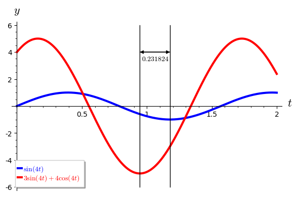
Solve the initial value problem

$\begin{equation*} y'' + 10y' + 29y = 0, \quad y(0) = 1, \quad y'(0) = 0 \end{equation*}$

🔗

(b)

Convert the solution to phase angle format and compute the phase angle $\theta$ in radians.

🔗

(c)

Plot both solutions in Task 4.5.2.a and Task 4.5.2.b on the same axis over the interval $[0,2]$ to confirm your analysis. What should you see?

🔗

Subsubsection Back to the Circuit

🔗

In our study of phase angle representation in the previous section we saw that the

$\sin(\omega t)$ and

$\cos(\omega t)$ terms of (4.5.4) can be combined into one sine term (albeit with a phase angle) with one amplitude,

$\begin{equation} \text{Amplitude}(y_{\text{steady state}}) = R \sqrt{\frac{C^{2} \omega^{2}}{C^{2} L^{2} \omega^{4} + {\left(C^{2} R^{2} - 2 \, C L\right)} \omega^{2} + 1}}.\label{secondorder05-equation-amplitude-steady-state}\tag{4.5.9} \end{equation}$

🔗

Thus, our gain (recall, gain is the ratio of the amplitude of the steady state output voltage,

$V_{\text{out}}\text{,}$ to the amplitude of the input voltage,

$V_{\text{in}}$ ) is

$\begin{equation*} \text{gain} = R \sqrt{\frac{C^{2} \omega^{2}}{C^{2} L^{2} \omega^{4} + {\left(C^{2} R^{2} - 2 \, C L\right)} \omega^{2} + 1}}. \end{equation*}$

🔗

Here,

$V_{\text{in}} = 1$ for

$E(t) = \sin(\omega t)$ and has amplitude

$1\text{,}$ which is a function of

$R\text{,}$

$L\text{,}$

$C\text{,}$ and

$\omega\text{.}$ Gain is a measure of the response of the circuit to input voltage

$E(t)\text{,}$ which in this case is

$E(t) = \sin(\omega t)\text{.}$

🔗

Let us fix

$R$ at

$1$ ohm and

$L$ at

$1$ henry and see what gain is in this case as a function of

$C$ over a range of

$\omega$ values. Let us “tune” this circuit by changing

$C\text{,}$ the size of the capacitance in the circuit and see how gain changes as input voltage frequency,

$\omega\text{,}$ changes.

plots of the gain with peaks at — 🔗
FigurePlot of gain as a function of input frequency, $\omega\text{,}$ for various values of capacitance, $C = 0.5\text{,}$ $0.05\text{,}$ $0.005\text{,}$ $0.0005$ farads in with $R = 1$ ohm and $L = 1$ henry.

🔗

Figure 4.5.4 illustrates the power of differential equation modeling. For we can alter parameters in our equation and see the results in a physical (in this case electrical) system. Indeed, we see in this plot that for a capacitance of

$C = 0.0005$ farads if we have an input voltage with a frequency around

$\omega = 45$ (

$44.7214$ to be precise) then the gain is greatest. Optimization is a calculus problem and we merely have to take the derivative of gain with respect to ω and find where it is

$0\text{.}$ All other frequencies give smaller gain for this particular capacitance. In fact, we can say that as we decrease our capacitance the optimal frequency; i.e., frequency which gives highest gain, decreases and we might want to look into this for a more exact relationship. We shall do that in Activity 4.5.3.

🔗

Put another way, we see that if our input voltage has a specific frequency,

$\omega\text{,}$ there is a unique capacitance,

$C\text{,}$ for this circuit that will maximize our gain. By changing

$C$ we can tune our circuit to maximize gain for a given input frequency,

$\omega\text{.}$ This is, in fact, how we tune a radio, for we change the capacitance of the radio's circuit so as to maximize the gain for the frequency (on our dial) that we wish to hear. So, the next time you try to find the station where Cousin Brucie is dedicating a Top Ten song from “Billie Bob” to “Sally May” know that a differential equation describes exactly what you are doing. How's that for cool?

🔗

Activity 4.5.3.

🔗

(a)

Use your understanding of RLC circuits to show for an imposed $E(t) = \sin(\omega t)$ on the RLC circuit given by

$\begin{equation*} L y'' + Ry' + \frac{1}{C} y = \omega \cos(\omega t), \quad y(0) = 0, \quad y'(0) = 0 \end{equation*}$

the maximum gain is obtained when $\omega = 1/\sqrt{LC}$ and thus we could tune our radio by changing the inductance $L$ as well, if that were as convenient as changing the capacitance, which it is not. So let us stick to tuning by changing the capacitance $C\text{.}$

🔗

Activity 4.5.4. Tune the Radio.

The Amplitude Modulated (AM) radio carrier frequencies are in the frequency range 535–1605 kHz. One Hz means $1$ cycle per second while kHz means $1,{}000$ cycles per second. The unit Hz is called a hertz. Carrier frequencies of 540 to 1600 kHz are assigned at 10 kHz intervals. The (Frequency Modulated (FM) radio band is from 88 to 108 MHz.²⁵ Recall 1 kHz means 1,000 cycles per second. So 660 kHz is oscillation at the rate of 660,000 cycles per second. We offer up a “radio”,

$\begin{equation} L \frac{dI^2}{dt^2} + R \frac{dI}{dt} + \frac{1}{C} I = E'(t),\label{secondorder05-equation-radio}\tag{4.5.10} \end{equation}$

where $E(t) = \sin(\omega t)\text{,}$ and ask you to tune in several stations by changing the capacitance and computing the optimal gain for these stations.

HyperPhysics. 2009. AM and FM Radio Frequencies. http://hyperphysics.phy-astr.gsu.edu/hbase/audio/radio.html Accessed 18 September 2016.

We will have to tell the circuit what initial current is present; i.e., $I(0) = 0$ usually until we turn the switch on and also we can presume there is no change in the current intially; i.e., $I'(t) = 0\text{.}$ Let us build this radio with the following values: $E(t) = \sin(\omega t)\text{,}$ $L = 0.033$ henrys, $R = 100$ ohms, and $C$ in farads can vary as needed to tune to various input frequencies $\omega\text{.}$ We note that if we wish to have, say 540 kHz, then $\omega = 540{,}000 \cdot 2\pi\text{,}$ and in general to have x kHz we will need $\omega = x \cdot 1000 \cdot 2\pi\text{.}$

🔗

(a)

Solve the differential equation (4.5.10) for the radio circuit.

🔗

(b)

Collect the coefficients $A$ and $B$ of the steady state $\sin(\omega t)$ and $\cos(\omega t)$ terms, respectively. Show that all other terms will dissipate, i.e. go to zero quickly, leaving only $\sin(\omega t)$ and $\cos(\omega t)$ terms.

🔗

(c)

Using the information above compute the gain as a function of capacitance $C$ and input voltage frequency $\omega\text{.}$

🔗

(d)

For a given input voltage frequency $\omega$ determine the maximum gain for this circuit.

🔗

(e)

For several AM frequencies, say 540 kHz ( $\omega = 540000 \cdot 2 \cdot \pi$ ), 880 kHz ( $\omega = 880000 \cdot 2 \cdot \pi$ ), and 1520 kHz ( $\omega = 1520000 \cdot 2 \cdot \pi$ ), plot gain as a function of the capacitance $C$ to demonstrate that your maximum gain is what your formula in Task 4.5.4.c predicts and that your radio is tuned in.

🔗

Subsection 4.5.2 Project—Hanging Mass and Rubberband

🔗

Subsubsection The History of the Tacoma Narrows Bridge

🔗

On July 1, 1940, the Tacoma Narrows Bridge was completed and opened to traffic (Figure 4.5.6). From the first day of operation, the bridge experienced vertical oscillations of several feet. The bridge received the nickname “Galloping Gertie” for its wild behavior. On the morning of November 7, the bridge began undulating up and down with motions as large as three feet. Later, the bridge began to experience torsional oscillations as large as 23 degrees. The bridge finally came crashing down at 11:10 a.m. For a long time, the collapse of the Tacoma Narrows Bridge was attributed to resonance. However, we shall soon see the the story is more complicated.

a photo of the original Tacoma Narrows bridge — 🔗
Figure 4.5.5. The Tacoma Narrows Bridge

🔗

Construction on first Tacoma Narrows Bridge, A.K.A. “Galloping Gertie”, was completed on July 1, 1940, the bridge was opened to traffic (Figure 4.5.6). Even on the first day of operation, people driving bridge experienced vertical oscillations of several feet. On the morning of November 7, these vertical oscillations were as large as three feet. Later that morning, the bridge began to experience torsional oscillations as great as 23 degrees. The bridge failed castrophically at 11:10 a.m. with the center span falling into Puget Sound below.

a photo of the second and third Tacoma Narrows bridges — 🔗
Figure 4.5.6. The Tacoma Narrows Bridge (2017)

🔗

There are many interesting stories connected with the first Tacoma Narrows bridge. One of the insurance policies had been written by a local travel agent who pocketed the premium and failed to report the $800,000 policy to his company. During sentencing at his trial, he pointed out that bridge officials had planned to cancel all policies in one more week after which his crime would have never been discovered. After the collapse of the Tacoma Narrows bridge, the governor of the State of Washington announced, “We are going to build the exact same bridge, exactly as before.” Theodore Von Kármán, director of the Guggenheim Aeronautical Laboratory at the California Institute of Technology and a member of the board of inquiry into the collapse,²⁶ sent a telegram to the governor stating, “If you build the exact same bridge exactly as before, it will fall into the exact same river exactly as before.”

The Jet Propulsion Laboratory, managed by the California Institute of Technology for the National Aeronautics and Space Administration grew out of the Guggenheim Aeronautical Laboratory.

🔗

Subsubsection The Design of the Narrows Bridge

🔗

The Tacoma Narrows bridge is a suspension bridge like the Golden Gate bridge. The road bed of the suspension bridge was hung from vertical cables attached to other cables strung between the two towers. If we think of the cables as long springs, it is tempting to model the oscillations of the road bed with an harmonic oscillator, and one's first guess as to the reason for the collapse of the bridge would be resonance.

🔗

However, the answer may not be so simple. If the collapse of the bridge was due to resonance, the forcing frequency of a forced harmonic oscillator must be close to its natural frequency, but the wind (the forcing) simply does not behave like this. One explanation might be the fact that cables are not true springs. They act more like rubber bands. Imagine a mass suspended by both a spring and a rubber band. The rubber band acts like a spring when it is stretched, but there is no restoring force if the oscillator is in a compressed position (Figure 4.5.7).²⁷

For the arguments for and against resonance, consult the references at the end of this section.

a mass hanging from a beam by both a spring and a rubber band — 🔗
Figure 4.5.7. A spring-rubber band system

🔗

Subsubsection The Spring-Rubber Band Model

🔗

Suppose that

$y(t)$ is vertical displacement of the mass the spring-rubber band model (Figure 4.5.7), where the displacement is positive in the downward direction and negative in the upward direction. We will also assume that we have a damped system. If this is the case, we can model the motion of the mass with the differential equation

$\begin{equation} my'' = - b y' - k_1 y - k_2 y^+ + F(t),\label{secondorder05-equation-spring-rubber-band-1}\tag{4.5.11} \end{equation}$

🔗

where

$y^+ = \max(y, 0)\text{.}$ Here,

$m$ is the mass,

$b$ is the damping coefficient,

$k_1$ is the spring constant, and

$F(t)$ is the forcing term. The term

$k_2 y^+$ corresponds to the rubber band in our system and can be explained as follows:

$\begin{equation*} y^+(t) = \begin{cases} y(t), & \text{the rubber band is stretched}, \\ 0, & \text{the rubber band is slack or tight but not stretched}. \end{cases} \end{equation*}$

🔗

Thus, the rubber band acts as a spring with spring coefficient

$k_2\text{,}$ if the rubber band is stretched, but has no effect on the system if the rubber band is slack. Of course, the term

$my''$ is just an application of Newton's Second law of Motion.

🔗

We can rewrite equation (4.5.11) in the more familiar form

$\begin{equation} my'' + b y' + k_1 y + k_2 y^+ = F(t),\label{secondorder05-equation-spring-rubber-band-2}\tag{4.5.12} \end{equation}$

🔗

Our first observation is that this equation is a nonlinear due to the

$y^+$ term. This may effect how sensitive the system is to initial conditions. A linear harmonic oscillator is not sensitive to initial conditions. For example, suppose we consider the harmonic oscillator

$\begin{equation*} y'' + 2 y' + 2y = \sin t \end{equation*}$

🔗

and examine the behavior of the solutions for different initial conditions. In Figure 4.5.8, we give the solutions for

$y(0) = 0$ with

$y'(0) = -4\text{,}$

$y'(0) = 1\text{,}$ and

$y'(0) = 3\text{.}$ Even though the transient part of the solution can differ a great deal depending on the initial conditions, all of the solutions eventually approach the steady-state solution.

solutions to a forced harmonic oscillator with different initial conditions and all converging to the same oscillating curve for large times — 🔗
FigureSolutions of $y'' + 2 y' + 2y = \sin t$

🔗

Let us return to our spring-rubber band model and let us assume that

$m = 1\text{.}$ We can rewrite equation (4.5.12) as a system of first-order equations,

$\begin{align*} y' & = v\\ v' & = - k_1 y - k_2 y^+ - b v + F(t) \end{align*}$

🔗

$\begin{align*} x' & = v\\ v' & = - h(y) - b v + F(t), \end{align*}$

🔗

where

$\begin{equation*} h(y) = \begin{cases} k_1 y & \text{if } y \lt 0 \\ (k_1 + k_2) y & \text{if } y \geq 0. \end{cases} \end{equation*}$

🔗

Let us assume that the forcing term is

$F(t) = 10 + \lambda \sin \mu t\text{.}$ If we keep

$\lambda$ small and assume that both

$y(0)$ and

$y'(0)$ are small, there will always be tension on the rubber band. Or in the case of the Tacoma Narrows Bridge, there will always be tension on the cables of the suspension bridge. However, a large initial velocity such as a gust of wind on the bridge, might cause the cables to go slack.

🔗

To see how this works in practice, we choose constants

$\lambda = 0.1\text{,}$

$\mu = 4\text{,}$

$k_1 = 13\text{,}$

$k_2 = 4\text{,}$ and

$b = 0.01\text{,}$ the system becomes

$\begin{align*} y' & = v\\ v' & = - h(y) - 0.01v + 10 + 4 \sin 0.1 t \end{align*}$

🔗

where

$\begin{equation*} h(y) = \begin{cases} 13 x & \text{if } x \lt 0 \\ 17 x & \text{if } x \geq 0. \end{cases} \end{equation*}$

🔗

This is a nonautonomous (and nonlinear) system and can be very sensitive to initial conditions. If we find a numerical solution to this system with

$y(0) = 0$ and

$v(0) = 4.764\text{,}$ we obtain low amplitude solutions (Figure 4.5.9). However, we only have to change the initial velocity of the system slightly to

$v(0) = 4.765$ in order to obtain large amplitude solutions that do not die out over time.

an oscillating position curve with the oscillations becoming smaller after an initial time span of large oscillations — 🔗
FigureInitial conditions $y(0) = 0$ with $y'(0) = 4.764$ and $y'(0) = 4.765$

an oscillating position curve with the oscillations remaining large for all times — 🔗
FigureInitial conditions $y(0) = 0$ with $y'(0) = 4.764$ and $y'(0) = 4.765$

🔗

Subsubsection The Bridge Model

🔗

We can now model the bridge by

$\begin{equation*} m y'' + \alpha y' + \beta y + \gamma y^+ = -gm + F(t), \end{equation*}$

🔗

where

$y$ is the height of the road bed at the center of the bridge.
$m$ is the mass of the bridge.
$\alpha y'$ is the damping term. We assume that $\alpha$ is small since suspension bridges are relatively flexible structures.
$\beta y$ is the force provided by the material of the bridge pulling the bridge back to $y = 0\text{.}$
$\gamma y^+$ is the force provided by the pull of the cables.
$-gm$ is the force provided by gravity.
$F(t)$ is the periodic force provided by the wind. Yes, wind does provide a periodic force. Just think of how a flag flutters in a wind.

🔗

Subsubsection The Model for Torsion

🔗

We have still not accounted for the large torsional oscillations that occurred on November 7, 1940, the day that the Tacoma Narrows bridge collapsed. If we look down the bridge (Figure 4.5.6), we see the road bed suspended from two cables—one on each side of the road. Thus, we can view a cross-section of the bridge as a rod suspended by cables or springs on each end. The bar is free to move vertically and rotate about its center of mass.

🔗

If a spring with spring constant

$k$ is extended by a distance

$y\text{,}$ the potential energy is

$ky^2/2\text{.}$ Let

$\theta$ be the angle of the rod from the horizontal. If a rod of mass

$m$ and length

$2l$ rotates about its center of gravity with angular velocity

$d\theta/dt\text{,}$ then its kinetic energy is given by²⁸

$\begin{equation*} \frac{1}{6} m l^2 \left( \frac{d \theta}{dt} \right)^2. \end{equation*}$

🔗

The potential due to gravity is

$-mgy\text{.}$

Consult your local physicist.

🔗

The extension of one spring is given by

$(y - l \sin \theta)^+$ and

$(y + l \sin \theta)^+$ in the other, where

$y^+ = \max(y,0)\text{.}$ We are making the assumption that the cables remain vertical. Since the cables are relatively long compared to the length of the roadbed, this is a reasonable assumption.

🔗

The total potential energy is given by

$\begin{equation*} V = \left(\frac{k}{2}\right) \left( \left( (y - l \sin \theta)^+\right)^2 + (y + l \sin \theta)^+ \right)^2 - mgy, \end{equation*}$

🔗

and the total kinetic energy is given by

$\begin{equation*} T = \frac{m}{2} \left( \frac{dy}{dt}\right)^2 + \frac{1}{6} m l^2 \left( \frac{d \theta}{dt} \right)^2. \end{equation*}$

🔗

Let

$L = T - V$ and put

$\begin{equation*} \frac{d}{dt} \left( \frac{\delta L}{\delta \theta'} \right) = \frac{\delta L}{\delta \theta} \end{equation*}$

🔗

and

$\begin{equation*} \frac{d}{dt} \left( \frac{\delta L}{\delta y'} \right) = \frac{\delta L}{\delta y} \end{equation*}$

🔗

where

$\delta \theta'$ and

$\delta y'$ are small damping terms. Thus, we obtain the equations

$\begin{align*} \frac{1}{3} m l^2 \theta'' & = k l \cos \theta [(y - l \sin \theta)^+ - (y + l \sin \theta)^+]\\ y'' & = -k [(y - l \sin \theta)^+ + (y + l \sin \theta)^+] + mg \end{align*}$

🔗

Since the force exerted by the springs (cables) is not perpendicular to the rod but at an angle

$\theta\text{,}$

$\cos \theta$ must appear in the first equation. Adding forcing and damping terms, we have

$\begin{align*} \theta'' & = - \delta \theta' + \frac{3k}{ml}\cos \theta [(y - l \sin \theta)^+ - (y + l \sin \theta)^+] + F(t)\\ y'' & = - \delta y' - \frac{k}{m}[(y - l \sin \theta)^+ + (y + l \sin \theta)^+] + g. \end{align*}$

🔗

If we assume that the cables never lose tension, then

$\begin{align*} (y - l \sin \theta)^+ & = y - l \sin \theta\\ (y + l \sin \theta)^+ & = y + l \sin \theta \end{align*}$

🔗

and we end up with the uncoupled equations

$\begin{align*} \theta'' & = - \delta \theta' - \frac{6k}{m}\cos \theta \sin \theta + F(t)\\ y'' & = - \delta y' - \frac{2k}{m} y + g. \end{align*}$

🔗

The first equation models the torsional motion while the second models the vertical motion.

🔗

If the torsional oscillations are very small, then we can assume that

$\begin{equation*} \sin \theta \approx \theta \qquad \text{and} \qquad \cos \theta \approx 1, \end{equation*}$

🔗

$\begin{align*} \theta'' & = - \delta \theta' - \frac{6k}{m}\theta + F(t)\\ y'' & = - \delta y' - \frac{2k}{m} y + g, \end{align*}$

🔗

each of which is which is linear. However, the torsional oscillations for the Narrow bridge were as large as 23 degrees. The linear model

$\begin{equation*} \theta'' = - 0.01 \theta' - (2.4) \theta + (1.2) \sin(0.06 t) \end{equation*}$

🔗

and the nonlinear model

$\begin{equation*} \theta'' = - 0.01 \theta' - (2.4) \cos \theta \sin \theta + (1.2) \sin(0.06 t) \end{equation*}$

🔗

behave very differently under the initial conditions

$\theta(0) = 1.2$ and

$\theta'(0) = 0\text{.}$ See Figure 4.5.10 and Figure 4.5.11

oscillating position and velocity curves with the same oscillations for all values of time — 🔗
Figure 4.5.10. Solution of the linear model for torsion

oscillating position and velocity curves that grow large for large values of time. — 🔗
Figure 4.5.11. Solution of the nonlinear model for torsion